BIOS 1 - Homework 1

Source code and data for this assignment

Note: The code used to create this document is here.

In this homework we will use the NHEFS dataset introduced in week 4. Take a look at the codebook linked to from https://www.hsph.harvard.edu/miguel-hernan/causal-inference-book/.

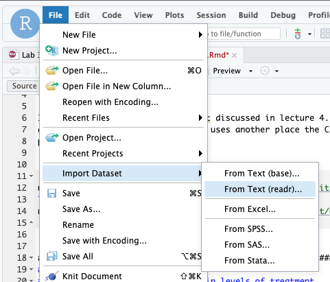
Download the dataset and import it into R. Try using the File - Import Dataset - From text (readr) menu option to do this import yourself.

Here is code to directly import the NHEFS dataset from the web. Note use of the knitr code chunk option cache=TRUE to cache the results locally and avoid downloading from the web each time you run your program.

library(readr)
nhefs <- read_csv("https://cdn1.sph.harvard.edu/wp-content/uploads/sites/1268/1268/20/nhefs.csv")

## Rows: 1629 Columns: 64
## ── Column specification ────────────────────────────────────────────────────────
## Delimiter: ","
## dbl (64): seqn, qsmk, death, yrdth, modth, dadth, sbp, dbp, sex, age, race, ...
## 
## ℹ Use `spec()` to retrieve the full column specification for this data.
## ℹ Specify the column types or set `show_col_types = FALSE` to quiet this message.

Question 1: customizing read_csv

Using help from the Import Dataset tool demonstrated above, change the above read_csv command to import any factor (categorical) variables in the first 15 columns as factors instead of double (numeric). You don’t need to recode their numeric values yet.

Question 2: recoding

You will use the following variables. For those that are factors, use the dplyr case_match function to recode them to informative factor levels. For yes/no factors use “no” as the reference category, and for other factors use whichever is the most common group as the reference category.

• active
• age
• education
• exercise
• race
• sex
• smokeintensity
• smkyrs
• wt82_71

Question 3: Table 1

Use the table1 package (or an alternative of your choice) to make a “Table 1” summarizing the above variables. Use the table1::label command to create informative labels for these variables in your table.

Question 4: draw a DAG

1. Use http://www.dagitty.net/ to create a DAG for the following hypothesis. Use the R dagitty package to display this DAG in your document:

• wt82_71 is caused by qsmk (in particular, that quitting smoking causes weight gain)
• sex, race, age, education, and exercise are hypothesized confounders.

2. Write out in words this research hypothesis, using the meanings of these variables rather than just their variable names.

3. Also write out in words the null hypothesis for statistical testing. Why would you have a two-sided null hypothesis even when in this case the research hypothesis is one-sided?

Question 5: fit a regression model

Fit the following multiple linear regression model (note that age squared is represented in model formula by I(age^2)):

$$wt82\_71 \sim qsmk + sex + race + age + age^2 + education + exercise$$

See https://www.oreilly.com/library/view/the-r-book/9780470510247/ch009-sec009.html for a convenient summary of how to use R model formulae.

Question 6: standardization

1. Calculate the mean predicted outcomes under treatment (quitting smoking) and no treatment (not quitting smoking).
2. Calculate the difference between these to estimate the causal effect of quitting smoking on change in weight.
3. Is the conditional average treatment effect that you estimated using standardization the same or different than the coefficient for qsmk in the table of regression coefficients?

Question 7: DAG and regression with interactions

Now suppose we hypothesize that smoking intensity also impacts weight loss, and modifies the effect of quitting smoking on weight loss.

1. Draw a new DAG that incorporates these hypothesized effects of smoking intensity.
2. Fit a new linear regression model that includes a linear and quadratic term for smokeintensity (as above with age) and an interaction between qsmk and smokeintensity.

Question 8: standardization with interactions

1. Again use standardization to calculate the conditional average treatment effect of quitting smoking in this sample.
2. Is this estimate the same or different than the coefficient for qsmk in the new table of regression coefficients from Question 7?

Question 9: bootstrap

1. Write a function that takes two arguments: function(x, d) where:

• x is a dataframe or tibble of your data
• d is an integer vector of row IDs that will be used to choose a subset of the dataframe, for example using dplyr::slice(x, d)

Using the subset dplyr::slice(x, d), your function should perform the same calculation as Question 8a, returning the conditional average treatment effect for the same model with the interaction term.

2. Show the output of calling your function using d = 1:nrow(x) to confirm that this gives the same result as 8a.

3. Estimate a 95% bootstrap confidence interval for the conditional average treatment effect, using at least 1000 replications. You are welcome to use your favorite method to implement this bootstrap, but I recommend the boot library which is powerful and simpler to use than programming your own simulation.

4. Summarize your findings. Is the effect of quitting smoking on weight change significant? What is the effect? Is it modified by baseline smoking intensity?

Question 10: what did those quadratic terms do?

Use the coefficients of age and I(age)^2 to plot the conditional relationship between age and weight change for the participants in this study. Specifically, use the ages of the participants in this study to calculate

$$y = \beta_{age} * age + \beta_{I(age)^2} * age^2$$ then create a scatterplot of y vs age. How did the quadratic term change the modeled association between age and weight change, compared to a linear term only?